source: http://arxiv.org/abs/2312.12141

Chapter 1: Causal Tyranny

Fried dopamine receptors. That’s the price we have to pay to live in a world where answers arrive faster than questions can be asked. We are so spoiled by instantaneity that we have stopped asking how the model knows or answers.

You type: “The capital of India is”

Before your finger finds it way away from the return key, Delhi materializes in front of your eyes. It feels like magic, it feels like telepathy. It feels like a lookup table.

But surprisingly enough, it’s none of the three. It’s something more fundamental, yet stranger: accumulation by simple, relentless vector addition.

Between the “is” and “Delhi,” exactly 33 different mathematical operations are fired across sixteen transformer layers. Billions of parameters dancing in tandem to the tune of matrix multiplications. Yet, somewhere in the cascade, exactly one specific operation probably outshone others and wrote the word “Delhi” into existence.

The other parameters/parameter groups were busy doing grunt work of maintenance: ensuring “Mumbai” is suppressed, sharpening context, and just marking attendance for a geography question that they don’t quite understand yet.

Question remains: which one was the author? in which layer the threshold reached certainty from maybe?

That is the tyranny of causality in deep networks. The output is deterministic, traceable, and mathematically inevitable. (cue iron man) Despite all this, the authorship remains an opaque layer.

We aare not dealing with a single body of “intelligence,” but with a committee of 33 vectors, each scribbling it’s “opinion” onto a shared “scratchpad.” This scratchpad is star of today’s show aka residual stream.

They pass the same page down the line, adding notes, crossing out errors, gradually building towards a consensus that none of them claim individually. By the final layer, the scratchpad contains not one voice but a superposition of 33 vector opinions to speak as one.

To find the guilty layer, we must learn to read the scratch pad.

Chapter 2: The Additive Heresy

There is no magic that happens here. No ghost in the layers (cue interstellar) guiding the model to the right answer and obviously, no secret lookup table of capitals buried under layer 11.

The residual stream, that we need to examine, operates on almost an insultingly simple principle: vector addition. That’s it. Just a clandestine dance floor in a high dimensional space and a choreography around a simple summation.

But before we commit to this heresy against the “mystique” of AI, we must bow to the architecture. The architecture is not the crime, it’s the canon.

The Residual Concept

In a standard function approximation, a layer learns the full mapping $Y=F(X)$. The residual stream, instead, learns the difference ie $F(X)=Y-X$, thereby reconstructing the output as $Y=X+F(X)$.

For the transformer architecture this means, we can define two “residuals” that let us take a peek into how the information is accumulated.

Attention Residual: $L_{res}\leftarrow L_{in}+ATTN(L_{in})$ This keeps the token representation, but adds contextual information.
FFN Residual: $L_{out}\leftarrow L_{res}+FFN(L_{res})$ This keeps the contextual representation and refines it further.

Now, this becomes crucial for two main reasons that makes the entirety of logit lense-ing and arguably, a large subpart of mechanistic interpretability possible.

Identity is always available: If the layer isn’t useful, network skips the learning using the skip or residual connections. The information flow remains unchanged by outputting zeroes.
Gradients flow directly by taking alternate paths. This prevents vanishing or exploding gradient catastrophes of deep architectures.

Without these skip/residual shortcuts, the layers and vectors wouldn’t be waltzing, they would be fighting for survival in a slaughterhouse, each dancer(layer) obliterating the momentum(information) from before. Thankfully, instead of this, we have accumulation.

The Stacked Pre-LN Doctrine

For our example, we’ll interrogate a 16-layer, decoder-only transformer operating under the Pre-LayerNorm constraints. Unlike archaic Post-LN designs where normalization acted as a censor at the end, the Pre-LayerNorm sanitizes the input before each operation. This ensures that the residual stream remains a raw, unnormalized and pure accumulation of information.

The canonical specifications:

16 cycles of accumulation(layers), each housing Multi-Head Attention(MHA) and Feed Forward Network(FFN)
Causal masking enforced absolutely, no precognition, no taking a sneak peek at the future.
The Pre-LN rite: $\hat{X} = LN(X)$ before projection, preserving gradient highways and identity.
4096 neurons per FFN layer: the individual neurons that are waiting to testify
8 simultaneous attention heads, each of 128 dimensions, projecting from the same sanctified input through distinct $W_{Q},W_{K},W_{V}$ matrices.

The forward pass follows this exact choreography:

$$\text{(Sanctification)}\quad\hat{X} = \mathrm{LN}(L_{\text{in}})$$

$$ \text{(Attention)}\quad \mathrm{Attention}(X) = \sigma\left(\frac{QK^{T}}{\sqrt{d_k}} + M_{\text{causal}}\right)V $$

$$ \text{(First Join)}\quad L_{\text{res}} = L_{\text{in}} + \mathrm{Attention}(X) $$

$$ \text{(FFN)}\quad \mathrm{FFN}(L_{\text{res}}) = \mathrm{ReLU}\big(\mathrm{LN}(L_{\text{res}})W_1 + b_1\big)W_2 + b_2 $$

$$ \text{(Final Join)}\quad L_{\text{out}} = L_{\text{res}} + \mathrm{FFN}(L_{\text{res}}) $$

The plus operator is the key here. Because of them, the stream $L_{in}$ stays immaculate, receiving additive amendments without corruption.

The Waltz of the Thirty-Three

It’s very easy to mistake the residual stream as a literal “stream” of flowing river. But that’s too fluid. The intuition we’re aiming for is a manuscript that is written and overwritten, again and again with every layer’s contribution still visible in the final manuscript.

Picture the residual stream as a clandestine dance floor of dimension $R^{d_{\text{model}}}$.

For the token “is” at position $t_{n}=5$ in our sentence “<start> The capital of India is”, the stream begins with an initial embedding $L_{in_{0}}^5$ which is a single vector claiming “I am the word ‘is’ preceded by the word ‘India’”.

Then the choreography executes.

Layer 0: attention adds contextual vectors. FFN adds refinement vectors.
Layer 1: Another pair of additions

…
Layer 15: The final set of additions.

For the $i^{th}$ layer and the $t_{n}^{th}$ token, in general,

$$L_{in_i}^{t_n} = L_{out_{i-1}}^{t_n}\qquad \text{input to layer } i \text{ for token } t_n$$

$$ L_{res_5}^{i} = L_{in_5}^{i} + \mathrm{ATTN}_5^{i} \qquad \text{residual after attention} $$

$$ L_{out_5}^{i} = L_{res_5}^{i} + \mathrm{FFN}_5^{i} \qquad \text{residual after feed-forward network} $$

This results in not a transformation but a superposition of the following:

$$L_{out_{15}}^5=L_{in_{0}}^5+\sum_{i=0}^{15}ATTN_{i}^5+\sum_{i=0}^{15}FFN_{i}^5$$

33 high dimensional vectors, all existing in the same high-dimensional space, each contributing to the same directional momentum. The “Delhi” token emerges as a vector sum of the:

$L_{in_{0}}^5$ -> the initial embedding
$\sum_{i=0}^{15}ATTN_{i}^5$ -> sum of the attention vectors which are the “contextual” redirects
$\sum_{i=0}^{15}FFN_{i}^5$ -> sum of the FFN vectors which are the “factual” shoves

Thirty three additions. One result. That’s the magic.

But this is not atomic yet. There’s one more layer that we can peel off this “information” inducing onion.

Each attention output itself decomposes into attention subvalues. These are individual contributions from each previous token position. There are 6 tokens here including the “start” token so 6 subvalues plus bias. $$ATTN_{i}^5 = \sum_{j=0}^{5} attn_i^{5,j} + attn_i^{b} \qquad \text{since sentence has 6 tokens, attention output for layer (i) is sum of 6 attention subvalues + a bias}$$
Each FFN output is a result of 4096 subvalues, where individual neurons fire or remain silent.

$$FFN_i^{5} = \sum_{k=0}^{4095} ffn_i^{k} + ffn_i^{b} \qquad \text{each FFN computed by adding 4096 FFN Subvalues and an FFN bias.}$$

After the subvalues are computed,

$$\text{(FFN)}\quad\mathrm{FFN}(L_{\text{res}}) = \mathrm{ReLU}\big(\mathrm{LN}(L_{\text{res}})W_1 + b_1\big)W_2 + b_2$$

this operation with ReLU enforces hard sparsity, ensuring that a lot of the 4096 neurons output zero, maintaining silence. However, attention operates as a soft routing mechanism, weighting contributions adequately rather than silencing them completely.

The Attention Alibi

Each of the 16 attention blocks can be further scrutinised. It’s a collection of contributions from every previous token position. For our 6 token sequence “<start> The capital of India is”:

$$ATTN_{i}^5 = \sum_{j=0}^{5} attn_i^{5,j} + attn_i^{b}$$

here, $attn_{i}^{5,j}$ denotes specific contribution from token $j$ eg “India” at $j=3$ to token $t=5$ at layer $i$.

The Architectural View

To trace the footsteps, we must reconstruct the scene of the crime.

We have established that the attention output $ATTN_{i}^5$ is a collection of subvalues, each representing a specific token’s testimony. But the process is unclear still.

How is each individual contribution $attn_{i}^{5,j}$ manufactured?

The Lineup

The architecture follows a clear, strict protocol:

Input: The sanctified residual stream vectors $X_{t}$ for tokens $t$=0 to 5 for our example.
Query for token: For token 5, the query would be $q_5^{h}=X_{5}W_{Q}^{h}$ -> denotes the question asked only for the current token, by the head $h$. $W_{Q}^h$ projects to the query vector.
Keys: $k_{j}^h=X_{j}W_{K}^h$ where j goes from 0 to 5.
Values: $V_{j}^h=X_{j}W_{v}^h$ where j goes from 0 to 5

The Interrogation

The scaled dot product is calculated to check for the compatibility, per head:

$$e_{5,j}^h=\frac{{q_{5}^{h}.k_{j}^h}}{\sqrt{ d_{k} }} \quad \text{where j goes from 0 to 5}$$

This score is then normalized by softmax into attention weights, to answer the question: “how much should token 5 trust token $j$ ?”

$$\alpha_{5,j}^{h}=\frac{\exp(e_{5,j}^h)}{\sum_{j’}{} \exp(e_{5,j’}^{h})} \quad \text{where the softmax runs over all six token positions}$$

The Verdict by a Single Head

for head $h$, the attention output is given by $head_{5}^h=\sum_{j=0}^5 \alpha_{5,j}^hv_{j}^h$ .

The Council - All the Attention Heads convene

We concatenate across all 8 heads:

$\alpha_{5}=[head_{5}^0||head_{5}^1||\dots||head_{5}^7]$

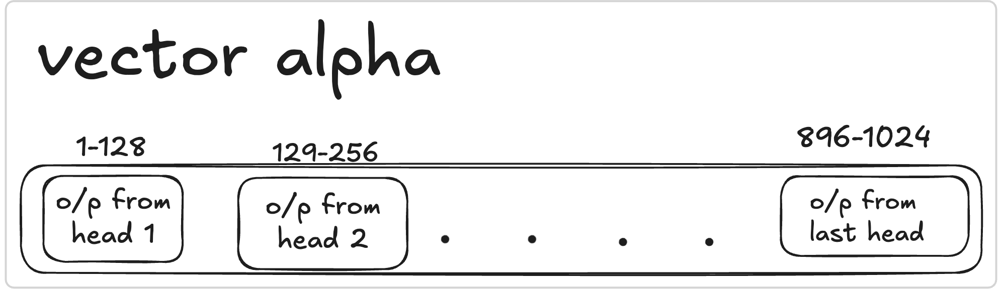
Multi-head attention architecture

The Final Report

Project the value back to the model dimension via $W_{O}$:

$attn_{5}=\alpha_{5}W_{O}$

Via a procedural chain of matrix multiplications and a bunch of linear transformations, we get the value of the attention. But, real eyes realize real lies. We need to see through the mechanism to do the true detective work of mechanistic interpretability.

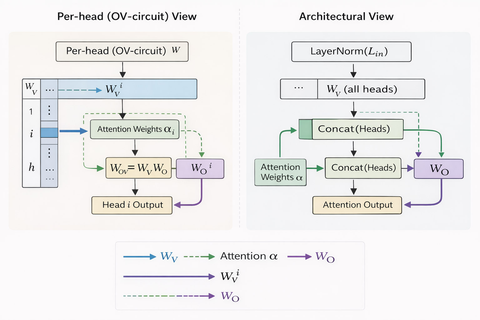
The Mechanistic View

Sleight of hand and a slight reordering of matrix multiplication yields in a more interpretable result.

We multiply by $W_{V}$, attend and then multiply by $W_{O}$ . But since they are linear transformations, reordering yields the same result. $$W_{OV}^{(h)}=W_{V}^{(h)}W_{O}^{(h)}$$

This “virtual weight” matrix reveals the net effect of the head, independent of how the attention is routed. It tells us clearly what information this head can write, regardless of the source.

Rewriting the head output using this decomposition,

$$attn_{5}^{(h)}=\sum_{j}{(\alpha_{5,j}^{(h)})} \cdot {(X_{j}W_{OV}^{(h)})}$$

this beautifully separates the concerns:

$\alpha_{5,j}^{(h)}$ : chooses the source
the OV circuit/matrix $W_{OV}$ chooses the content

An intuitive way to think of it is: $W_{OV}$ prepares a “feature template,” that can potentially be copied from any position.

The attention weights simply vote on which positions supply that template.

One head might have learnt “geographical entities.” The attention weights determine that “India” in position 3 is the relevant entity for this context.

Another head might copy “capital city” relationships.

Mechanistically,

$X_{j}$ is the residual stream vector at position j
$W_{OV}^{(h)}=W_{V}^{(h)}W_{O}^{(h)}$ the OV matrix determines what kind of feature the head can write into the residual stream
$\alpha_{5,j}^{(h)}$ determines which tokens supply that feature
sum it over j and aggregate information from multiple positions

Per head vs architecture

The weights simply determine where to look for that specific relational information.

[!note] Attention chooses the source. OV chooses the content. The same linear transformation applied to every source token. Attention scales how much each transformed token contributes.

For our “Delhi” investigation, we can ask two distinct questions that can narrow it down for us:

Which previous tokens contributed most to the prediction?
What kind of information was being copied?

In the chosen model, with 8 heads of 128 dimensions each, we have eight distinct $W_{OV}$ matrices, each capable of writing a different “genre” of feature into the residual stream.

The Memory Palace: FFN Subvalues

If attention is the process of referral, then FFN is the mechanism of recollection, retrieving facts from the model’s parametric memory.

While attention subvalues, are calculated dynamically from the context, the FFN subvalues are purely static parameters: knowledge frozen during training, activated when the right pattern appears in the residual stream.

Each neuron $k$ in the $i^{th}$ layer operates as a conditional statement: “If i detect pattern X, i shall write feature Y to the stream.”

At layer $i$, token 5 (“is”), the residual stream at that point is denoted by $L_{res_{i}}^5$ .This contains a superposition of everything learned so far.

the grammatical structure “capital of”
geographical entity “India”
syntactic position that requires completion.

The FFN layer “interrogates” this vector through 4096 specialized detectors, each waiting for a specific pattern. This is the key-value memory mechanism. it happens in a two phased manner.

Consider neuron $k$ that has learned the pattern “capital of [COUNTRY]“

1. Detection

Here, the neuron calculates a coefficient score.

$$m_{i}^k=ReLU(LN(L_{res_{i}}).FC1_{i}^k+b_{i}^k) \quad \text{answers: is my feature present in the input?}$$

here,

$LN(L_{res_{i}})$ is the current state of knowledge in the residual stream
$FC1_{i}^k$ is the key. This is the pattern detector pointing in a specific direction of the high dimensional space. Here, it might point in the direction of “capital-city-query” patterns.

If the normalized residual stream aligns with this direction, meaning that the the context of the residual stream strongly matches with the pattern “capital of [COUNTRY]”, then the dot product yields a high positive value.
$ReLU$ simply thresholds it to zero if the pattern is absent.

2. Writing

If activated, i.e., $m_{i}^k>0$ , the neuron writes that value into the residual stream. The neuron writes its value into the stream:$$FFN_{i}^k={m_{i}^{k}}\cdot{FC2_{i}^k} \quad \text{if feature present in input, then add this information vector to the stream}$$

For our capital-city neuron, $FC2_{i}^k$ is the value. This vector contains the directional components towards “Delhi,” “Beijing” and other capitals, with “Delhi” being strongly represented because India was mentioned in this context.

This is not merely a lookup table, but a vector “nudge”, wherein the neuron adds a weighted version of $FC2_{i}^k$ to the residual stream, nudging the representation towards the subspace where “Delhi” lives.

The sparsity is brutal: out of 4096 available, only 50-100 fire for the specific input.

one neuron might detect the “capital of” pattern
another detects “India-as-geography”
another detects “south asia”

… and this combined detections create the composite vector that eventually points to “Delhi.”

The Matrix Structure

The $W_{1}$ matrix ( $d_{\text{model}}\times 4096$ dims) contains all the $FC1^k$ vectors as its columns.

Thousands of question-askers basically scan simultaneously for different queries/patterns, asking questions like “Is this a number?” “is this future tense?” and for our case, “Is this a capital-city query?”

The $W_{2}$ matrix ($4096 \times d_{\text{model}}$ dims) contains all the $FC2^k$ vectors as its rows. These are the answers waiting to be spoken out loud. When the detection scores $m_{i}$ (a sparse vector of length 4096) multiply $W_{2}$ , we select only the rows corresponding to the firing neurons.

Thus, for the sentence “The capital of India is,” the FFN performs a brutal but elegant operation: it scans the residual stream for thousands of patterns simultaneously, finds the few that match (capital-city, India, geography), and adds their associated fact-vectors to the stream, incrementally building the case for the answer being “Delhi” in the final output.

Chapter 3: The Forensic Timeline

Now that we have established the architecture of the crime with the residual stream acting as the scratchpad, attention as the referral mechanism and FFN as the memory palace.

Now that we have all the essential components, let’s compose the timeline.

For token 5 (here, “is”), what exactly happens at layer $i$ and how does each vector addition nudge the vector towards the goal (here, “Delhi”)?

Step A: The Lineup

At the start of layer $i$, the residual stream $L_{in_{i}}^5$ contains the accumulated wisdom of all previous layers. This includes:

the word “is”
the context of “capital”
the geography of “India”

This is done by the attention mechanism, which now conducts a lineup of all previous tokens(token 0 through 5). Consider an attention head that specializes in “geographical attribution.” It projects a query vector from the current token “is”: $$q_{5}^h=LN(L_{in_{i}}^5)W_{Q}^h \quad \text{asks: What country are we discussing?}$$

Each previous token $j$ projects a key vector $k_{j}^h=LN(L_{in_{i}}^j)W_{K}^h$.

The token “India” at position 3 produces a key that strongly aligns with the geographical query, yielding a high attention weight $\alpha_{5,3}^h$ after the softmax normalization.

The value vector $v_{3}^h=LN(L_{in_{i}}^3)W_{V}^h$ contains the contextual representation of “India.”
This is then retrieved and scaled by $\alpha_{5,3}^h$ .
Through the OV circuit mechanism that we saw #The Mechanistic View, this writes a vector into the stream that effectively says: “The current position is semantically bound to India.”

For a simpler example, “Apple announced new products,” a different attention head at this same stage would look back at position 0 (“Apple”).

By comparing it’s query against the keys of surrounding tokens like “announced” and “products”, it detects a corporate context rather than a “botanical” or “fruity” sense.

The head writes a contextual update that shifts the residual vector away from the fruit subspace and towards the “technology” company subspace.

Thus, attention does not retrieve facts about Apple, it just updates the pointer to “indicate” which “sense” of the word is active.

The result, thus, enters the residual stream as:

$$L_{res_{i}}^5=L_{in_{i}}^5+{ATTN_{i}^5}$$

Step B: Total Recall

The contextually enriched vector $L_{res_{i}}^5$ enters the feed-forward network, our vast memory palace, where parametric knowledge resides. Attention routes information from other position while FFN retrieves facts stored directly in its weights.

The mechanism, as we saw, involves a key-value memory with hard sparsity. Each neuron performs a detection (the key in #1. Detection) followed by writing to the residual stream (the value in #2. Writing). This is not a database lookup but a vector addition: the neuron adds a weighted version of its knowledge vector to the residual stream.

For our “Delhi” investigation, imagine the $k^{th}$ neuron detecting the “capital of India” pattern.

It’s $FC2$ vector points strongly towards “Delhi” in the embedding space. When activated, it adds to the residual stream: “The answer is Delhi.”

Step C: The Amendment

The FFN output is added to the residual stream:

$$L_{out_{i}}^5=L_{res_{i}}^5+FFN_{i}^5=L_{in_{i}}^5+ATTN_{i}^5+FFN_{i}^5$$

This is strictly cumulative. The token representation now carries the following information:

the original embedding
a contextual update pointing to “India” (from attention)
a factual vector pointing to “Delhi” (from FFN)

The “Delhi” component is scaled by the neuron’s confidence $m_{i}^k$ .If the pattern was weak, it corresponds to a mathematical whisper. If strong, it’s a scream to the right answer.

Step D: Passing the Baton

The vector $L_{out_{i}}^5$ now enriched with both contextual and factual retrieval becomes $L_{in_{i+1}}^5$ for the next layer.

The process repeats, layer by layer adding more specific information, with the final layer finalizing the confidence mass required for prediction.

Chapter 4: The Mathematics of Accumulation

We have described the dance. We have understood the choreography. Now let’s measure the steps with mathematical precision.

The most crucial property of residual connections makes it reproducible and easy to scale as well: each update is a simple vector addition, not a functional transformation.

Thus, $L_{out}=(L_{in}+\text{some update})$ instead of $L_{out}=f(L_{in},\text{some update)}$ as we see in #The Residual Concept.

The Linear Ledger: Before-Softmax Values

When we add a vector $v$ (a layer’s contribution) to vector $x$ (representing the current residual state), the change in the before-softmax(BS) value or the logit value for any token $t$ is strictly linear as $$(x+v).{e_{t}}=x.e_{t}+v.e_{t}$$ where $e_t$ is the un-embedding vector for token $t$.

So, here $x.e_t$ represents the old score and $v.e_t$ represents the change.

Let’s define $bs_t^x=x.e_{t}$ as the before-softmax value, giving us the linear evidence that we are looking for.

The Proportional Evidence

To get proper evidence, we must understand how each choice influences the outcomes.

So for the same embedding matrix $E$, each vector is mapped to a vocabulary space as $V \in \mathbb{R^B}$

The probabilities, with softmax, are:

$$p(t|x)=\frac{{\exp(e_{t}\cdot x)}}{\sum_{j=1}^{B}\exp(e_{j}\cdot x)}$$

$$p(t|v)=\frac{{\exp(e_{t}\cdot v)}}{\sum_{j=1}^{B}\exp(e_{j}\cdot v)}$$

$$p(t|x+v)=\frac{{\exp(e_{t}\cdot (x+v))}}{\sum_{j=1}^{B}\exp(e_{j}\cdot (x+v))}$$

Now,

$$p(t \mid x+v)= \frac{\exp(e_t \cdot (x+v))}{\sum_{j=1}^{B} \exp(e_j \cdot (x+v))}= \frac{\exp(e_t \cdot x + e_t \cdot v)}{\sum_{j=1}^{B} \exp(e_j \cdot (x+v))}= \frac{\exp(e_t \cdot x)\exp(e_t \cdot v)}{\sum_{j=1}^{B} \exp(e_j \cdot (x+v))}$$

$$$$

This reveals a proportionality relation.

$$p(t|x+v) \propto {\exp(e_t \cdot x)\cdot\exp(e_t \cdot v)}$$

The new probability, thus, depends on the product of two exponentials:

the original evidence for $t$ (stored in $x$)
the new evidence introduced by $v$

However, while it’s very fundamental, it’s easy to get lost in the intuition and not notice that the proportionality obscures the competition.

The denominator sums over all tokens ie $v$‘s effect on token $t$ depends NOT JUST on $e_t.v$ but on how $e_t.v$ compares to every other $e_k.v$.

A better question to ask would be: How much larger is $e_w.v$ than other $e_k.v$ values?

Assuming $v$ creates a uniform distribution where the dot product with all embeddings yields the same value, it adds no discriminative signal.

However, if $v$ creates a skewed distribution, ie high alignment with some tokens, negative with others, it acts as a selective amplifier.

The Before Softmax Spectrum

For any vector $v$ , we can examine it’s BS spectrum across the entire vocabulary as:

$$bs(x)=[bs_{1}^x,bs_{2}^x,\dots bs_{t}^x,\dots bs_{B}^x]$$

The spectrum reveals the vector’s true “intentions”. When we add $v$ to $x$, the effect on token $t$ follows a conditional logic:

if $bs_{t}^v$ is among the highest in the spectrum ie strongly positive, then, adding to $v$ will increase the probability of token $t$.
if $bs_{t}^v$ is among the lowest, ie strongly negative, then adding $v$ will decrease probability of token $t$.
if $bs_{t}^v$ is in the middle range then the effect depends on the baseline distribution of $x$.

The conditional behavior explains why a single neuron can contain multitudes. The neuron’s value vector $FC2_i^k$ mgiht have moderately high dot products with “cold,” “winter,” “frost” and “snow.” However, it’s not dominant for any single token. Instead, it collectively nudges the distribution towards the subspace containing winter concepts.

Thus, one neuron may encode many useful features simultaneously. It’s contribution distributed across the semantic field rather than concentrated on a single word.

The Voting Mechanism

Tying this back to our FFN memory palace: when neuron $k$ detects its pattern and fires with a “strength” coefficient of $m_i^k$ , it writes $FFN_{i}^k=m_{i}^k.FC2_{i}^k$ into the stream. The resulting change to token $t$‘s score is:

$$\quad\text{Change = }m_{i}^k.FC2_{i}^k$$

For example, a neuron detecting “royalty” might have:

$FC2.e_\text{King}$=+5.0
$FC2.e_\text{apple}$=-0.2
$FC2.e_\text{Queen}$=+4.8

When this neuron fires with strength $m_{i}^k$=0.8, it adds exactly +4.0 to King’s logit and +3.84 to Queen’s. it votes up it’s allies and ignores the irrelevant result, ie apple, in our example. The coefficient $m_{i}^k$ acts as the “voting weight” which basically says how hard the neuron pushes its “agenda.”

Thus, we can calculate exactly how much a specific neuron changes the score of a specific word through the simple dot product. This is independent of the non-linear probability calculations that follow.

The Softmax Trap

The investigation gets tricky here. We care about the probabilities, not just the raw scores. But the probabilities are non-linear. The softmax function:

$$p(t|x)=\frac{{\exp(e_{t}\cdot x)}}{\sum_{j=1}^{B}\exp(e_{j}\cdot x)}$$

creates a zero-sum battlefield of sorts. Adding a vector $v$ that boosts both “King” and “Queen” might seem beneficial for both.

But if Queen surges faster than King, King’s actual probability percentage might shrink due to normalization. The competition matters more than the individual intent.

This pertains to quantifying the contributions of a layer/module for predicting the next word. Mathematically, contribution of vector $v$ when adding on to vector $x$ to predict token $t$.

Calculating the contributions

With the example of “<start> The capital of India is”, the probability increase of input token “is” on the $6^\text{th}$ layer is given by difference of two states:

The BEFORE comprises of $L_{in_6}^5$ which is basically input to layer 6 for token position 5. This is the state of the model BEFORE layer 6 has contributed anything. In other words, what the model knows up to end of layer 5. It represents a hypothetical state in the latent space where the layer says: “I know that we’re talking about a country and it’s capital but not sure which state. I have a gut feeling it’s Delhi with 10% confidence.”
The AFTER comprises $L_{res_{6}}^5$ which is basically the output from layer 6 for token position 5. This contains the residual information added by the layer 6’s attention heads and FFN layer. This represents a hypothetical state in the latent space saying: “I just looked back at the word ‘India’ and ‘capital’ and I’m pretty sure the next word is ‘Delhi’ with about 80% confidence.”

The delta is the direct contribution:$$p(\text{“Delhi”|}L_{res_{6}}^5)-p(\text{“Delhi”|}L_{in_{6}}^5)$$ which can alternatively be read as,

$$p(\text{“Delhi”|}\text{After Layer 6 for token 5})-p(\text{“Delhi”|}\text{Before Layer 6 for token 5})$$

This checks the direct contribution of layer 6 to the correct prediction “Delhi”, essentially answering the question: did layer 6 figure out the answer or did it already know the answer?

If the delta is large and positive for layer 6, then it’s the hero: it added critical evidence to point to the right subspace. If the delta is near zero, layer 6 either inherited the solution(not the answer, the difference is crucial here) or remains as confused as before.

Logit Lensing

The operation $p(\text{“Delhi”}|x)$ is a logit lens, an investigatory tool that allows us to treat the intermediate vector $L_{in}$ or $L_{res}$ as if it were the final output, to reveal what the model would be guessing right now. It allows us to take a sneak peek into the scratchpad at any point in computation and ask: “What would the model guess right now?”

By projecting these intermediate states onto the unembedding matrix E, we can:

Blame specific layers for wrong turns, for example, if the probability of “Mumbai” spikes at layer 8 .
Credit specific layers for correct insights for correct insights, for example, if the probability of “Delhi” jumps at layer 6, ie $p(\text{“Delhi”|}L_{res_{6}}^5)-p(\text{“Delhi”|}L_{in_{6}}^5)\gg 0$

The Funky Function $F(l)$

The method of quantification holds good, but it has one flaw hiding in plain sight. It only becomes apparent when we interrogate the lower layers. We observe a two-step selection prediction process:

The Silent Sort: In early layers, the correct token’s probability stays low while its rank shoots up. The model knows “Delhi” is a candidate and maybe shows up in the top-50 guesses. However, it assigns it a very small probability mass. It’s a suspect, not a culprit.
The Loud Jump: Suddenly, at any given intermediate layer, a single vector v pushes the token’s score past a critical threshold, causing its probability to spike from 5% to 80%. The layer seems to have worked magic, when in fact it merely provided the final nudge.

This is not some divination. It’s pure math. Consider the funky function that governs the jump.

When adding vector $v$ with $BS(v)=[0,0,\dots,bs_{t}^v,\dots,0]$ with $p(t|v)=1$ ie a vector $v$ that ONLY cares about token $t$, the probability becomes:$$p(t|x+v)=\frac{{\exp(bs_{t}^x+bs_{t}^v)}}{\exp(bs_{t}^x+bs_{t}^v)+\sum_{i=1}^{\text{vocabulary}-{token}}bs_{i}^x}$$

From this, we can conclude that $v$ is helpful for increasing probability of token $t$ when $bs_t^v$ is greater than all other BS values.

This can easily be converted to a sigmoid-like form:

$$F(l) = \frac{A e^{l}}{A e^{l} + B}$$

where,

$$A = \exp(bs_{t}^x)\quad\text{strength of the correct token before boost}$$

$$B = \sum_{i=1}^{\text{vocabulary-{token}}} \exp(bs_{i}^x)\quad\text{combined strength of all competitors}$$

$$l = bs_{t}^v \quad \text{the boost provided by the layer}$$

Additionally, for sake of completeness,

$$x \quad \text{state of the residual before the jump}$$

$$v \quad \text{the update vector that was added to the layer}$$

$$t \quad \text{the correct token}$$

Now, if we plot the function, it becomes very easy to see the behavior.

Probability function curve

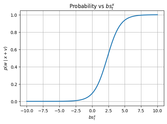
In the lower layers, $A\ll B$. This causes the correct token to be drowned out and lost in the crowd.
For small $l$ , $e^l \ll B$. $F(l)\approx{0}$
Only when $A.e^l$ approaches $B$ does this probability explode.

We might be wondering what’s the utility of having lower layers not boost the probability. However, the lower layers perform the “crucial” sorting step by pushing “Delhi” up the ranks without showing significant gain in probability. It is unfair to use raw probability increase as the contribution score, because it penalizes the early detectives and rewards only the one who closed the case, essentially.

The Logarithmic Remedy to Funkiness

However, the curve of $\log(F(l))$ is approximately linear. Wait, that rings a bell. What else uses log probability? Yep, the loss function during training. This makes this metric both fair and optimization relevant.

Log probability curve

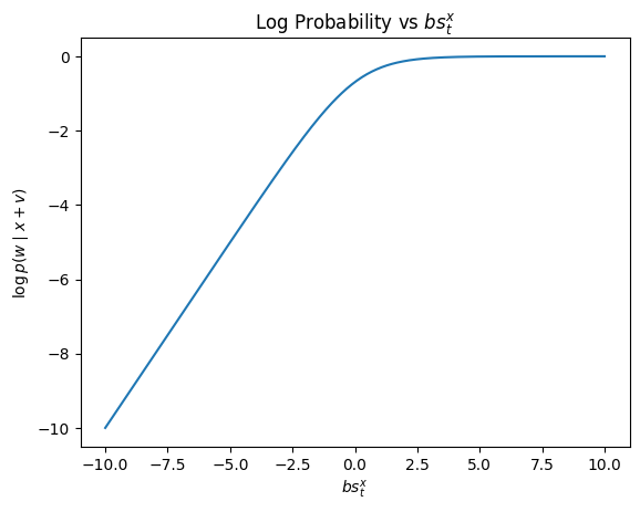
Thus, we can define a contribution metric/score $C(i)$ for layer $i$ predicting word $w$ as:

$$C(i)=\log(p(w|L_{i}))-\log(p(w|L_{i-1})) \quad \text{where }L_{i}\text{is the new vector after adding the layer’s vector}$$

So, we have:

$$C(ATTN_{6})=\log(p(L_{res_{6}}))-\log(p(L_{in_{6}}))$$ and $$C(FFN_{6})=\log(p(L_{out_{6}}))-\log(p(L_{res_{6}}))$$

This gives us an additive, interpretable measure of each layer’s contribution. This is irrespective of it acting early or late.

Now, this begs an important question: is there any relation amongst the contribution scores?

The Additivity of Evidence

We have defined the contribution scores using log probabilities. But do these scores play harmoniously together? By this, we mean, to predict token $t$ when vector $v$ is added to $x$, given we have $C(v_{1})$ and $C(v_{2})$ then what is $C({v_{1}}+{v_{2}})$?

Answer is, empirically, YES. When we rank all subvalues of an FFN layer by their contribution scores and accumulate them in ascending order -> calculating $C(v_1)$, then $C(v_{1}+v_{2})$, then $C(v_{1}+v_{2}+v_{3})$ and so on.

We observe a roughly linear relationship between the sum of individual scores and the score of the sum.

$C(v_{1})+C(v_{2})+⋯≈C(v_{1}+v_{2}+…)$

This validates our decomposition. The contributions are indeed additive, allowing us to treat the residual stream ass a “ledger” where each sub-value casts an independent vote for the final prediction.

Cross Layer Attribution: The Conspiracy OR Attribution Chains: Who activated Whom?

However, one thing we have to keep in mind is that layers aren’t insulated from each other. They conspire and work together to get the results.

An FFN neuron at layer 10 fires based on $L_{res_{10}}$, which in itself is the sum of the initiall embedding plus all the previous attention and FFN outputs. Is there any way to trace credit backward through this chain?

This mechanism is hidden in plain sight in the activation function. Recalling, $$m_{i}^k=ReLU(LN(L_{res_{i}}).FC1_{i}^k+b_{i}^k)$$

For activated neurons, the LayerNorm can be expanded. Grouping the multiplicative and constant terms, we see:

$$m_{i}^k=\frac{{L_{res_{i}}.K_{i}^k}}{V}-\frac{{E\lambda_{k}}}{V}+B_{i}^k$$

where,

$K_i^k=LN_{w}FC1_{i}^k$ is a fixed direction for that neuron
$\lambda_{k}$ is sum of all dimension scores of $K_{i}^k$
$B_{i}^k=LN_{b}.FC1_{i}^k+b_{i}^k$

For each FFN subvalue, $K_{i}^k$ and $B_{i}^k$ are fixed. The only thing changing are $L_{res_{i}}$ and consequently $E$ and $V$. In the equation, we can see that the bias term is heavily dominated by the numerator of $\frac{{L_{res_{i}}.K_{i}^k}}{V}$. Thus, if the dot product is strong, the neuron fires strongly, otherwise weakly.

To find which part of the residual stream switched the neuron on, we calculate the inner dot product $\text{Score}=\text{Vector}.K_{i}^k$ where vector maybe the output from an attention head.

Each term in the sum of $L_{res_{i}}=L_{res_{i}}=L_{in_{0}}+ATTN_{0}+FFN_{0}+\dots+ATTN_{i}$ contributes to the dot product that “switches on” the neuron. Thus each lower layer’s subvalue acts as a “query” to activate upper layer FFN coefficients.

Coefficient Score Accounting

We can perform credit-sharing, ie a group of layers/neurons coming together to contribute to a prediction. Suppose $L_{in}$ has a coefficient score of 2 and $ATTN$ has a score of 1 in the pre-LN state, for a total of 3.

Roughly, $L_{in}$ gets 2/3 of the final activation and $ATTN$ gets 1/3. However, the non linearity of LN means that this is a very fair approximation, not an certainty.

By calculating these inner products, we can answer: If the final score for “Delhi” is 4, how much came from the input stream and how much came from attention?

We can trace which specific attention head in layer 3 provided the clue that activated the “capital city” neuron in layer 8.

Chapter 5: Conclusion

We have followed the 33 vectors from the initial embedding to the final prediction. We have seen how:

attention heads act as witnesses, referring to past tokens for context
how FFN neurons serve as the memory palace, retrieving facts through key-value lookup
how logit lens lets us read the scratchpad at any point, assigning credit or blame with surgical precision

But this investigation isn’t just an academic exercise in reverse engineering. It’s foundational.

What this unlocks

If the residual stream is truly a scratchpad, and if “Delhi” truly emerges as a sum of discrete traceable vector additions, then we have unlocked a superpower. We can interrogate models in real time. We can now ask not just what a model predicts, but the why and how of predicting it, layer by layer, neuron by neuron.

This enables:

Automated circuit discovery: Instead of hand annotating which heads matter for which tasks, we trace high contribution sub-values algorithmically, mapping the functional circuitry of large models without grueling manual inspection.
Mechanistic Steering: If we know that a neuron $k$ in the $8^{th}$ layer adds a vector pointing towards “Delhi” then we can amplify or suppress that specific component, steering predictions without needing to retrain the entire network.
Anomaly detection: When a model hallucinates or generates malicious output, we can pinpoint exactly which suvalue introduced the error.

Expanding The Frontier: From Autopsy to Surgery

Currently, we perform autopsies. We feed a complete sentence, trace backward to see who “wrote” “Delhi” into the stream. The next frontier is “surgery”: intervening mid-streaming, patching specific vectors and observing how the distribution for the final prediction changes.

The techniques outlined here, including logit lensing, contribution scoring and cross layer attribution, all scale surprisingly well. They apply to behemoth 96-layer architectures as well. The residual stream still remains a sum of subvalues, be it made up of 33 vectors or 193. The challenge is not the math, but the search space. With billions of neurons, we need automated methods to bring to light the high-contribution candidates.

There is also a question of polysemanticity. Here, we assume each neuron $k$ detects “capital of {country}” but the reality is messier. Neurons often encode superpositions of unrelated features, their meanings often context dependent and distributed.

Additive Heresy Revisited

We began with a simple elusive mystery: how does a model know that Delhi is the capital of India?

We end with an answer that’s almost insulting in its simplicity. There is no dark arts involved. No ineffable gestalt of neural weights. There is only accumulation.

As it turns out, vector addition is all you need after all. Vector upon vector, scribble after scribble, until the page points decisively towards a single word.

The residual stream is but a manuscript. Every edit remains visible in the final text. To read it, all you need is $Y=X+F(X)$. The model doesn’t learn the full mapping, just the difference, just a nudge to the truth.

In demystifying the transformer, we do not diminish it. We make it accountable. And making it accountable means opening the door to building systems that we can understand, interpret, trust and steer.

The scratchpad is there. The scribbles are now legible. Case closed.

On This Page