Residual Streams - Notes
On This Page
- WHY residual stream?
- questions worth asking:
- architecture used
- Residual Stream
- Sub-value Residual Stream
- Understanding where and when these residuals happen
- where does it sit in the architecture?
- when does it happen?
- Mechanism analysis
- how distribution changes for the residual connections
- how does this connect back?
- Answering the questions now
- conclusion
source: http://arxiv.org/abs/2312.12141
Imagine peeking inside GPT’s brain, mid-prediction, and seeing which layer exactly says “Delhi” for the query “capital of India.” That’s sounds almost as complicated as performing a brain surgery and figuring out which neurons are firing to answer a query. what
Transformers feel like a black box, doing some kind of magic with the inputs. That is, only until we start asking a specific set of questions.
- how does the model know the answer to the fact that the capital of india is delhi?
- which exact layer amongst hundreds of layers or which parameter amongst billions does the fact reside in?
- which part of the network decided that the answer is delhi instead of mumbai or kolkata?
We’ll zoom into the layers and figure out the core idea that makes these questions answerable: the residual stream(ta-da!). This is a single vector/token that EVERY attention head and every FFN layer reads from and writes to, via simple vector addition, something very similar to a “scratchpad.” The mental model would be that instead of each layer replacing the token representation, it scribbles small updates onto the same page(residual stream). By following the scribbles, we can see which layers AND even which individual neurons contributed to the final answer.
To start off, we’ll see visualise residual stream first, then take a dive into the transformer and see how attention and FFN act as two very different kind of writers to the residual stream scratchpad. Attention gives more of the “where” to get the information to write into the scratchpad whereas FFN behaves like key-value pair of memories that detect patterns and add appropriate facts.
Once we’ve built the foundations along with the math, we’ll connect how the vector updates to changes in next token probabilities as well as a simple nifty way to quantify the contribution of each layer.
At the end of this blog, we’ll be able to:
- look at residual vectors and read off what token the model is leaning towards.
- quantify exactly how much a particular layer/neuron bumped up the logit of the correct next token.
- how “knowledge” is stored in FFN value vectors and routed by attention and LayerNorm through layers, rather than being trapped in a single layer.
- build a mental model of the residual stream as a cumulative vector highway, where every update is a linear addition that is retraceable.
there’s a little mechanistic goal that we are trying to achieve here, stay tuned for that.
WHY residual stream?
let’s think of residual stream as the information highway with layers being ramp-ups or ramp-downs to add or remove information. the residual stream serves two essential purposes:
- accumulation of information
- communication between layers
questions worth asking:
- where are important parameters containing the knowledge stored?
- are the important parms in one layer or many layers
- if we locate the most contributing layer/s, are they stored only in specified place like FFN modules?
- how to quantify the contribution score of a layer or module for predicting next token?
- how do parms contribute to prediction?
- do they directly store knowledge or contribute by activating other useful parms?
- if some parms directly contain knowledge, what is main mechanism to to merge knowledge into final embedding for prediction?
- are there any evident features of these parameters?
architecture used
- transformer layer: MHA+FFN
- layer norm CAN added to output or input of each module, but here, focus only on pre-LN arch.
- decoder only, medium sized.
- in attn mods,
- given input hidden states, $$X \in \mathbb{R}^{n \times d_{\text{model}}}$$
- LayerNorm first because Pre-LN $$\hat{X} = LN(X)$$
- $Q,K \text{ and } V$ from same normalized input $$Q = \hat{X}W_{Q}$$$$K = \hat{X}W_{K}$$$$V = \hat{X}W_{V}$$
- Causal masked attention $$Attention(X) = \sigma\left( \frac{QK^T}{\sqrt{d_{k}}}+M_{causal} \right)V$$
- Residual connection: $$X \leftarrow X+Attention(X)$$
- 16 transformer layers
- 4096 subvalues in each FFN
Residual Stream
- residual stream has proven useful for mech interp
called residual because:
-
instead of learning the full mapping $Y=F(X)$,
-
the model learns the residual $F(X)=Y-X$ reconstructing it to $Y=X+F(X)$
-
for transformers, the attention residual $L_{res}=L_{in}+Attention(L_{in})$ tells us “keep token representation, but add contextual(attention) information”
-
for transformers, the FFN residual $L_{out}=L_{res}+FFN(L_{res})$ means “Keep the contextual representation but refine it non linearly”
-
why crucial?
- identity always available. so if layer isn’t useful, network can skip learning.
- gradients flow directly allowing for alternate paths for the flow, resulting in no vanishing or exploding gradients.
-
here, we focus on both attn+FFN modules to analyse the whole residual stream
$$[L_{in_{0}},L_{res_{0}},L_{out_{0}}, \dots L_{res_{15}},L_{out_{15}}]$$
where $L_{in}$ and $L_{out}$ -> layer input and layer output OF ONE TRANSFORMER LAYER
$$L_{res_{i}}^{t_{n}} = L_{in_{i}}^{t_{n}}+Attention_{i}^{t_{n}}$$
this basically says that $L_{res}$ is the sum of $L_{in}$ and the $Attention$ output for that particular layer for that particular token.
so, for a sentence like $\text{{“
for the output stream of the token “is” with token position $t_{n}=5$ since $t_{n}$ for $
so for the $i^{th}$ layer and the $t_{n}^{th}$ token, in general,
$$L_{in_i}^{t_n} = L_{out_{i-1}}^{t_n}\qquad \text{input to layer } i \text{ for token } t_n$$
$$L_{res_5}^{i} = L_{in_5}^{i} + \mathrm{ATTN}_5^{i}\qquad \text{residual after attention}$$
$$L_{out_5}^{i} = L_{res_5}^{i} + \mathrm{FFN}_5^{i}\qquad \text{residual after feed-forward network}$$
the final layer(16) output would be given by $L_{out_{15}}^5$ -> used for predicting the next token
$L_{out_{15}}^5$ $\leftarrow$ sum of 33 vectors.
33 vectors -> $L_{in_{0}}^5$ which is the $0^{th}$ layer input from last layer of previous token + 16 attention outputs + 16 FFN outputs
Sub-value Residual Stream
- the residual stream “shows” the entire change amongst the layers.
- the attention and FFN outputs can also be calculated as “subvalues” of the residual stream.
Attention Subvalues
$$ATTN_{i}^5 = \sum_{j=0}^{5} attn_i^{5,j} + attn_i^{b} \qquad \text{since sentence has 6 tokens, attention output for layer (i) is sum of 6 attention subvalues + a bias}$$ $$FFN_i^{5} = \sum_{k=0}^{4095} ffn_i^{k} + ffn_i^{b} \qquad \text{each FFN computed by adding 4096 FFN Subvalues and an FFN bias.}$$
ReLU activation makes many FFN subvalues to not be activated.
While ReLU in the FFN enforces a hard sparsity by suppressing the inactive neurons, attention on the other hand operates as a soft routing mechanism over token posn. The attention weights $\alpha_{t,j}$ do not deactivate value vectors but instead determine how strongly each token contributes to the o/p via a weighted sum.
The attention subvalues are computed by:
$$attention_{i}^{5,0}=(\alpha_{i}^{5,0}(LayerNorm(L_{in_{i}}^0)V_{i}))W_{O}^i$$
architectural view
Step by step:
-
input: layer inputs $X_t$ for tokens $t$ = 0 to 5 for a 6 token sequence.
-
Query for token 5: $q_5^h=X_{5}W_{Q}^{h}$ where head $h$ and $W_{Q}^h$ projects to the query vector. used only for current token.
-
Key: $k_{j}^h=X_{j}W_{K}^h$ where j goes from 0 to 5.
-
Values: $V_{j}^h=X_{j}W_{v}^h$ where j goes from 0 to 5
-
Attention scores calculated per head $h$: $$e_{5,j}^h=\frac{{q_{5}^{h}.k_{j}^h}}{\sqrt{ d_{k} }} \quad \text{where j goes from 0 to 5}$$
and then $$\alpha_{5,j}^{h}=\frac{\exp(e_{5,j}^h)}{\sum_{j’}{} \exp(e_{5,j’}^{h})} \quad \text{where the softmax runs over all six token positions}$$
tells us “how much should token 5 read from token j in head h?”
-
attention o/p from a single head: $head_{5}^h=\sum_{j=0}^5 \alpha_{5,j}^hv_{j}^h$ across all tokens
-
Multihead attention:
vector concatenation across ALL heads $\alpha_{5}=[\alpha_{5}^{0} \dots \alpha_{5}^h]$ for h attention heads.
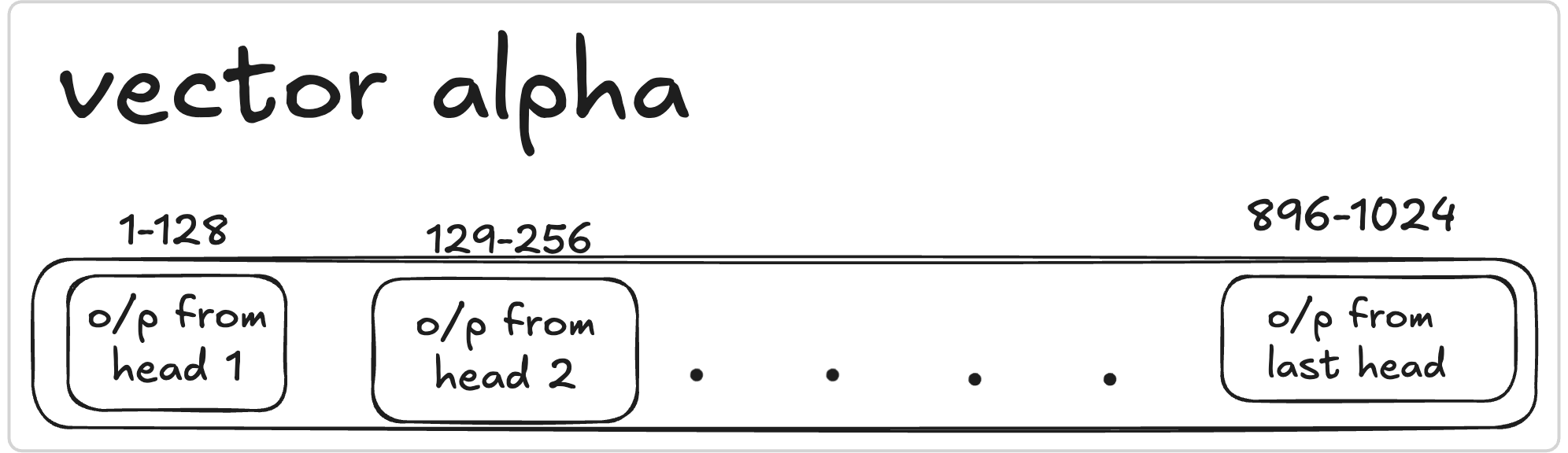
- Output projection: project via $W_{O}$ the output matrix for $0^{th}$ head.
$attn_{5}=\alpha_{5}W_{O}$
This is the architectural view.
mechanistic view
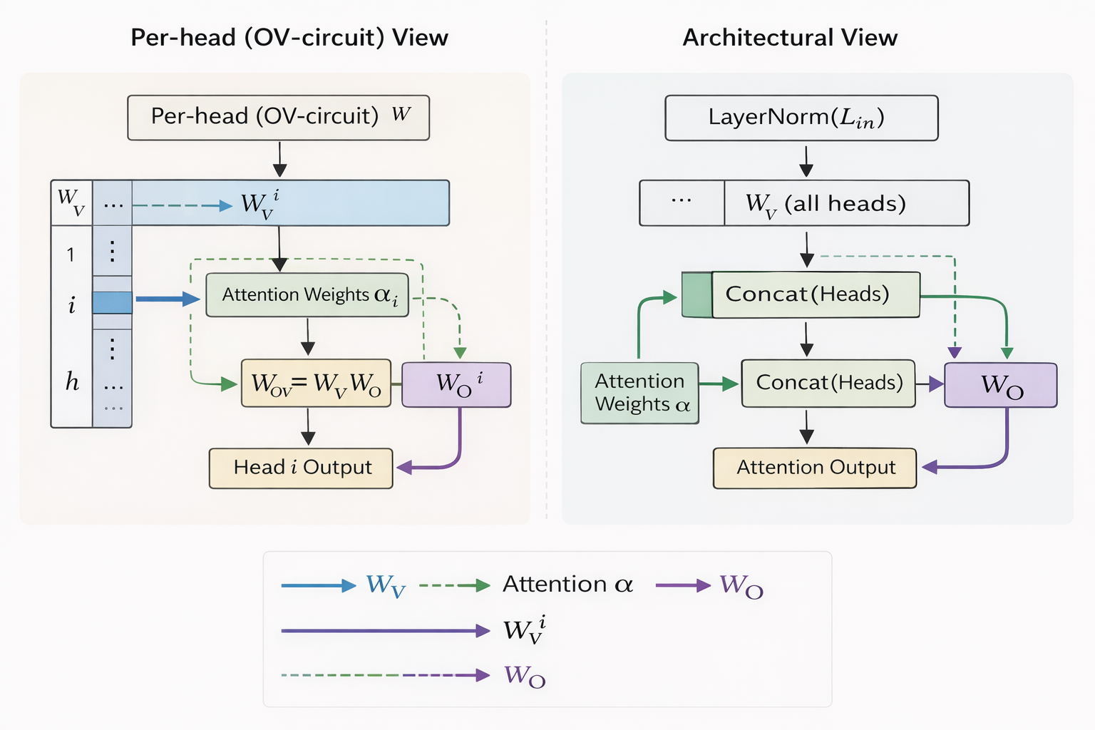
However, if we want the mechanistic view, we go by the OV Circuit analysis method:
- Since $W_{v}$ and $W_{o}$ are linear, they can be regrouped for interpretation as:
$$attn_{5}^{(h)}=\sum_{j}{(\alpha_{5,j}^{(h)})} \cdot {(X_{j}W_{OV}^{(h)})}$$
- Standard approach: multiply by $W_{V}$ -> get values V -> do attention -> multiply result by $W_O$ . gives order of ops for forward pass
- since $W_{V}$ and $W_{O}$ both linear matrices applied in sequence to the i/p, one single “virtual weight matrix”, given by $W_{OV}^{(h)}=W_{V}^{(h)}W_{O}^{(h)}$ describes net effect of head on the data.
- the OV matrix defines what info a head can write while attention defines where it writes from.
The formula can additionally be interpreted in two ways:
- for each head h and query token 5,
- each source token j produces a contribution
- that contribution is first linearly transformed by the head’s OV matrix $X_{j}\to X_{j}W_{OV}^{(h)}$ and then weighted by how much token 5 attends to token j.
- the final head output is the sum of all these weighted contributions
- mechanistically,
- $X_{j}$ is the residual stream vector at position j
- $W_{OV}^{(h)}=W_{V}^{(h)}W_{O}^{(h)}$ the OV matrix determines what kind of feature the head can write into the residual stream
- $\alpha_{5,j}^{(h)}$ determines which tokens supply that feature
- sum it over j and aggregate info from multiple positions
Info
attention chooses the source OV chooses the content the same linear transformation applied to every src token attention scales how much each transformed token contributes “writing a specific feature into the residual stream, copied from positions selected by attention”
in the chosen model, dims of $\alpha$ is 1024, heads dims is 128 and 8 heads in total. (128x8=1024)
FFN Subvalues
$FFN_{i}^k$ -> $k^{th}$ FFN subvalue on layer $i$(transformer block number) i.e contribution of $k^{th}$ neuron in the FFN of layer $i$
$FCn_{i}^k$ ->second matrix/fully connected layer inside the ML of Transformer block number i
key value memory mechanism
every neuron $k$ acts as: “if observe pattern x, feature y added”
steps:
- detection:
- the neuron has to be activated or deactivated. calculates a coefficient score $m_i^k$$$m_{i}^k=ReLU(LN(L_{res_{i}}).FN1_{i}^k+b_{i}^k) \quad \text{answers: is my feature present in the input?}$$
- the $LN(L_{res_{i}})$ denotes the current state of token -> the normalized residual stream ie what the model knows about the token thus far.
- pattern $FN1_{i}^k$ that serves as the “key” or “pattern detector”. shows the specific direction in the high dimensional space that the neuron $k$ is looking for. eg. neuron k might be looking for the word “bank” in a river’s context. dot pdt checks for similarity. $b_i^k$ is simply the bias term.
- ReLU after that to do thresholding and thus, $m_{i}^k$ tells us how confident the neuron is.
- writing:
-
the $FC2_{i}^k$ is the information. “value” or the “content”, the actual vector associated with the neuron. eg. if “river”+“bank” detected, then this vector MIGHT contain contextual info like “boat”,“soil” etc.
-
we take the info vector $FC2_{i}^k$ and multiply that with the detection score.
if high detection, strong version of the feature added.
-
$$FFN_{i}^k={m_{i}^{k}}\cdot{FC2_{i}^k} \quad \text{if feature present in input, then add this information vector to the stream}$$
Understanding where and when these residuals happen
where does it sit in the architecture?
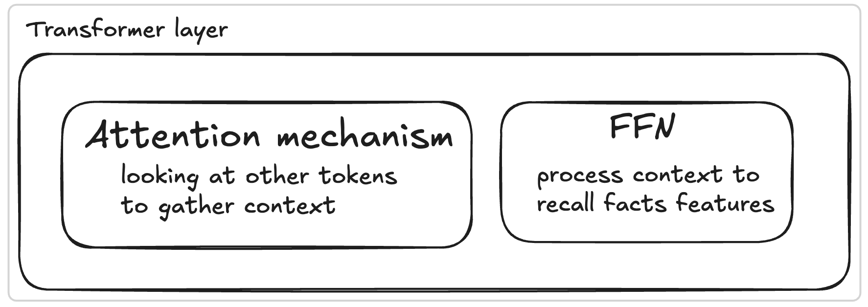
when does it happen?
Step A: Attention
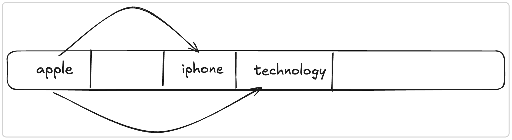
for eg,
- in a sentence, “apple” tends to “iphone” and “technology” elsewhere in the sentence.
- updates the vector to reflect the context, making the vector now mean “Apple” as the company and not the fruit.
- Result-> vector enters the residual stream $L_{res_{i}}$
Step B: Total Recall, the FFN
- the vector from residual stream enters FFN
- linear normalization to convert $\mu=0$ and $\sigma=1$
- pattern matching allows thousands of neurons to scan THIS vector
- neuron $n_1$ detects apple as “tech company” and crosses the threshold and fires. thus neuron fires when $m_{i}^{n_{1}}>0$
- neuron $n_{2}$ detects apple as “fruit” and doesn’t fire
- information retrieval for the neuron that fired ie for neuron $n_1$ here. so, it retrieves the vector that stores info about apple being a tech company ie info like “iphone, macbook, steve jobs”
how does the “recall” happen?
using the two massive weight matrices $W_1 \text{ and }W_{2}$ also known as $W_{in}\text{ and }W_{out}$ . they are the mathematical manifestations of the “keys” ie $FC1$ and “values” ie $FC2$.
- $W_{1}$
- holds all the patterns the layer knows how to recognize.
- dims: $\text{model dims} \times \text{hidden dims}$ . so for GPT 2 it’s 768x3072
- cols are “keys”. each col from the matrix is $FC1^k$ vector.
- so, when $LN(L_{res_{i}}).FN1_{i}^k$ this dot product is being calculated, what we’re doing is asking $\text{hidden dims}$ ie 3072 questions simultaneously as to whether the input vector look like pattern 1 or pattern 2 … or pattern 3072.
- $W_{2}$
- holds the features/facts that the layer can add to the residual stream
- dims: $\text{hidden dims} \times \text{model dims}$
- rows are “values”. each row is the $FC2^k$ vector.
- so, when the hidden state ie the scores $m^k$ are multiplied by $W_2$, we are SELECTING the rows corresponding to the neurons that are activated and adding them up to get the enriched output.
overall: $W_1$ maps input to pattern and $W_2$ maps pattern to information to enrich the input.
Step C: Update
- FFN output added to the original token vector to steer it in the right direction
- as a result, in our example, the token vector now represents “apple, maker of iphone and tech company”
Step D: Next Layer
The token vector, enriched by information, moves to the next layer $i+1$
Mechanism analysis
how distribution changes for the residual connections
each vector is a direct sum of other vectors rather than a function of it.
so, $c=a+b$ rather than $c=f(a+b)$. also a characteristic of the subvalue residual stream.
what we are trying to achieve: how o/p distribution in vocab space changes when vector x added to vector v.
so, for the same embedding matrix $E$, each vector is mapped to vocabulary space as $V \in \mathbb{R^B}$ so, for each token $t$, the probabilities (with softmax) are:
$$p(t|x)=\frac{{\exp(e_{t}\cdot x)}}{\sum_{j=1}^{B}\exp(e_{j}\cdot x)}$$
$$p(t|v)=\frac{{\exp(e_{t}\cdot v)}}{\sum_{j=1}^{B}\exp(e_{j}\cdot v)}$$
$$p(t|x+v)=\frac{{\exp(e_{t}\cdot (x+v))}}{\sum_{j=1}^{B}\exp(e_{j}\cdot (x+v))}$$
here, $e_{t}$ is the embedding of token $t$.
Now,
$$ p(t \mid x+v) = \frac{\exp(e_t \cdot (x+v))}{\sum_{j=1}^{B} \exp(e_j \cdot (x+v))} = \frac{\exp(e_t \cdot x + e_t \cdot v)}{\sum_{j=1}^{B} \exp(e_j \cdot (x+v))} = \frac{\exp(e_t \cdot x)\exp(e_t \cdot v)}{\sum_{j=1}^{B} \exp(e_j \cdot (x+v))} $$ so, $$p(t|x+v) \propto {\exp(e_t \cdot x)\cdot\exp(e_t \cdot v)}$$
however, other tokens not taken into account.
a fair argument is that the probability change is related to how much larger $e_{w}.v$ is larger than other tokens $e_{k}.v$ for a vector $v$ that has same probability on every vocab token.
so, what we essentially want to answer is: how much distribution change happens when we add $v$ and go from $p(w|x)$ -> $p(w|x+v)$?
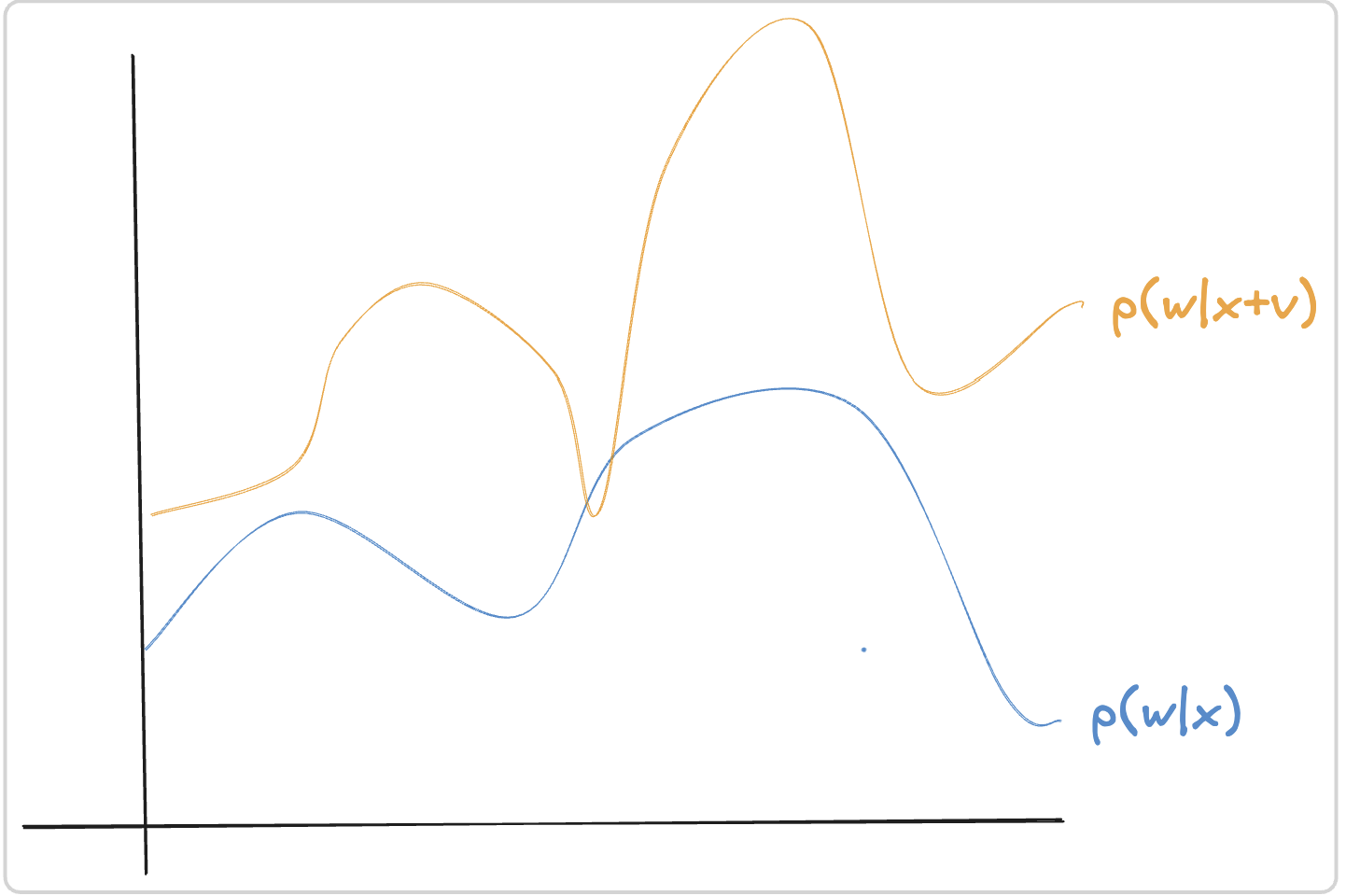
since $bs_{t}^x=e_{t}.x$ is the dot product of embedded token $t$ with the vector $x$, it’s called before softmax value of token $t$.
for both x and v, a token’s BS value corresponds to the probability and rank of this token.
so, for all vocabulary, the BS values are:
$bs(x)=[bs_{1}^x,bs_{2}^x,\dots bs_{t}^x,\dots bs_{B}^x]$ . so, if the largest value for vector $x$ is $t^{th}$ token with $bs_t^x$, the probability and rank of word/token $t$ will be the highest.
thus, if $bs_{t}^v$ is one of the highest bs values, then adding vector $v$ will increase probability on token t.
ie for vector v, probs of tokens with largest bs values will increase when adding $v$ on $x$ and for smallest bs values, probs of tokens will decrease when adding $v$ on $x$.
However, if it’s neither too large nor very small, then the changed distrib depends on prob of distrib of x.
thus, one neuron may contain many useful features.
how does this connect back?
Tying this back to the FFN residual values,
- we add vectors together for the residual connection
- we can calculate exactly how much a specific neuron changes the score of a specific word
- if FFN adds a vector $v=FFN_{i}^k$ to the stream input $x$,
- New Stream=$x+v$
- for token $t$
$$\text{New Score}= (x + v)\cdot e_t= x \cdot e_t + v \cdot e_t = \text{Old Score} + \text{Change}$$
for the equation $FFN_{i}^k={m_{i}^{k}}\cdot{FC2_{i}^k}$ ,
if $m_{i}^k>0$, then it enhances the probabilities of top bs value tokens in $FC2_i^k$ vector.
this is because:
- recall how $FC2_i^k$ basically contains features that can be added to the stream.
- this naturally aligns with some words and doesn’t with others. for eg it might point towards “cold” “winter” “snow”
- the coefficient $m_i^k$ tells us how “strongly” to push in that direction.
So, the top BS value tokens will be the ones that $FC2_i^k$ likes or gravitates towards.
this is because there’s a high positive dot product with $FC2_i^k$
eg something like $FC2 \cdot e_{\text{King}} = +5.0$.
now, since $m_i^k>0$, we add a positive amount, specifically $m_i^k \times 5$, resulting in the probability of “King” going up.
Analogy: This neuron detects a pattern and immediately votes to increase the likelihood of the specific words associated with that pattern.
Therefore, distribution change is caused by a direct addition function on BS values.
the change on probabilities caused by $v$ is non linear. so can’t predict using probabilities
- probabilities calculated using softmax, which is non linear.
- for eg, adding vector that tends to a certain word like “King” doesn’t guarantee that probability of only King goes up. another word like “Queen” might go up so fast, that King shrinks(since softmax, so has to add up to 1).
however, BS values or logits can be used to predict.
- linear relation. New Score=Old Score+Neuron’s addition
- since softmax preserves rank ie if a BS value significantly increases with respect to others, we can guarantee that its probability will eventually increase.
- therefore, by analyzing the highest BS value tokens in the added vector $v$, we can say which tokens the neuron is trying to promote.
Answering the questions now
part 7: if some parms contain knowledge, what is main mech to merge the knowledge into the final embedding for prediction?
this can be easily answered by the fact that if:
- subvalue contains knowledge
- then corresponding tokens will have high BS vals
- thus increasing probs when adding subvalue on other vectors
thus, this begs the 3rd question: how to quantify the contribution of a layer/module for predicting next word? i.e. contribution score of vector $v$ when adding on vector $x$ to predict token $t$.
calculating score
with the same example, of “<start> The capital of India is”,
the probability of increase of input token “is” on the $6^{th}$ layer is given by:$$p(\text{“Delhi”|}L_{res_{6}}^5)-p(\text{“Delhi”|}L_{in_{6}}^5)$$
can alternatively be read as:
$$p(\text{“Delhi”|}\text{After Layer 6 for token 5})-p(\text{“Delhi”|}\text{Before Layer 6 for token 5})$$
it checks the direct contribution of a part of the model (here, layer 6) to the correct prediction (“Delhi” the capital of India), essentially answering the question: did layer 6 figure out the answer or did it already know the answer?
before
$L_{in_6}^5$ -> input to layer 6 at posn 5
-
the state of the model BEFORE layer 6 has contributed anything ie what the model knows up to end of layer 5.
-
it represents a hypothetical state in the latent space where the layer says:
” i know that we’re talking about a country and it’s capital, but not sure which state. i have a gut feeling it’s Delhi with 10% confidence”
after
$L_{in_{6}}^5$ -> output from layer 6 at posn 5
-
state of the model AFTER layer 6 has contributed. contains residual information added by layer 6’s attention heads.
-
represents a hypothetical state in the latent space saying:
“i just looked back at the word ‘India’ and ‘capital’. I’m not pretty sure the next word is ‘Delhi’ with about 80% confidence.”
logit lens
This operation, $p(\text{“Delhi”}|x)$ is the “logit lens”. let’s us take a peek into what the logit says.
- takes an intermediate vector $x_{intermediate}$ like $L_{in}$ or $L_{res}$.
- considers that THIS is the final o/p of the model
- projects it to the vocab using the unembedding matrix to see what word the model would be GUESSING RIGHT NOW.
This technique let’s us blame or credit a particular layer for the predictions.
-
if $p(\text{“Delhi”|}L_{res_{6}}^5)-p(\text{“Delhi”|}L_{in_{6}}^5)\gg 0$ then we can say that the specific layer contributed to getting the information “Delhi” and wrote the answer “Delhi” to the residual stream.
-
if it’s $p(\text{“Delhi”|}L_{res_{6}}^5)-p(\text{“Delhi”|}L_{in_{6}}^5) \approx 0$ , then layer 6 didn’t do much.
it can either mean that model knew it already from prev layer OR doesn’t know it yet.
how to quantify the contributions?
but this method of quantifying the contribution has a bit of a disadvantage as well(for lower layers). Observation: two step prediction process during prob change:
- “silent” sort: the correct token prob stays low but rank shoots up. the model knows it’s a candidate but doesn’t commit to that token as the correct one yet.
- “loud” jump: a single layer adds vector $v$ that pushes that token’s score high enough to dominate the denominator, allowing it to spike in confidence.
- this also explains how a particular layer seemingly suddenly boosts the confidence rather than gradually increment.
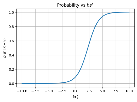
funky function
to understand why this happens, consider adding $v$ to $x$ in which $BS(v)=[0,0,\dots,bs_{t}^v,\dots,0]$ and $p(t|v)=1$. then the probability of $x+v$ is: $$p(t|x+v)=\frac{{\exp(bs_{t}^x+bs_{t}^v)}}{\exp(bs_{t}^x+bs_{t}^v)+\sum_{i=1}^{\text{vocabulary}-{token}}bs_{i}^x}$$
$v$ helpful for increasing probability of token $t$ when $bs_{t}^v$ is greater than other bs values.
$$F(l) = \frac{A e^{l}}{A e^{l} + B}$$ where,
$$ A = \exp(bs_{t}^x), \quad
B = \sum_{i=1}^{\text{vocabulary-{token}}} \exp(bs_{i}^x), \quad
l = bs_{t}^v
$$ $x$=state of residual stream before the “jump”
$v$=the update vector added by the layer
$t$=the correct token
$bs_{t}^x$=logit of the correct token before update
$bs_{t}^v$=boosted logit aded by vector v
- Thus, here
- A becomes the “strength” of the correct token before the boost
- B becomes the “sum of strengths” of all other tokens in the vocabulary.
- $e^l$ is the boost provided by the layer.
- think of $e^l$ as a boost given by the layer.
- for small $l$, $e^l \ll B$. Prob $\approx$ 0
- once $A.e^l$ gets close to $B$, the probability explodes.
- for large $l$,$e^l \gg B$. Prob $\approx$ 1
generally, A$\ll$B on lower layers as predicted token’s BS val is usually very very small on the first layer(how we can’t predict with much confidence that the next token is “Delhi” given the token “is”).
since it increases only after a point, not fair to use the prob increase as the contribution score. for upper layer, it’s more than the lower layer.
log of funky function
however, the curve of $\log(F(l))$ is linear. it’s equal to the loss function during training as well. double benefit.
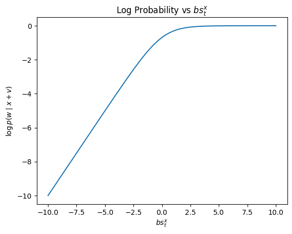
the log probability increase gives us the contribution score $C(i)$ for the $i^{th}$ layer for predicting word $w$. $$C(i)=\log(p(w|L_{i}))-\log(p(w|L_{i-1}))$$ where, $L_{i}$ is the new vector after adding the layer’s vector.
so, for the sake of completion,
$C(ATTN_{6})=\log(p(L_{res_{6}}))-\log(p(L_{in_{6}}))$ and $C(FFN_{6})=\log(p(L_{out_{6}}))-\log(p(L_{res_{6}}))$
is there any relation among contribution scores?
by this, we mean, to predict token $t$ when vector $v$ is added to $x$, given we have $C(v_{1})$ and $C(v_{2})$ then what is $C({v_{1}}+{v_{2}})$?
-
we rank all suvalues of one FFN layer by their contrib scores
-
calculate sum in ascending order ie $[v_{1},v_{1}+v_{2},v_{1}+v_{2}+v_{3},\dots]$
-
then we calculate $C(v_{1})+C(v_{2})+C(v_{3})$ and $C(v_{1}+v_{2}+v_{3})$
-
there’s a roughly linear relationship between contribution scores
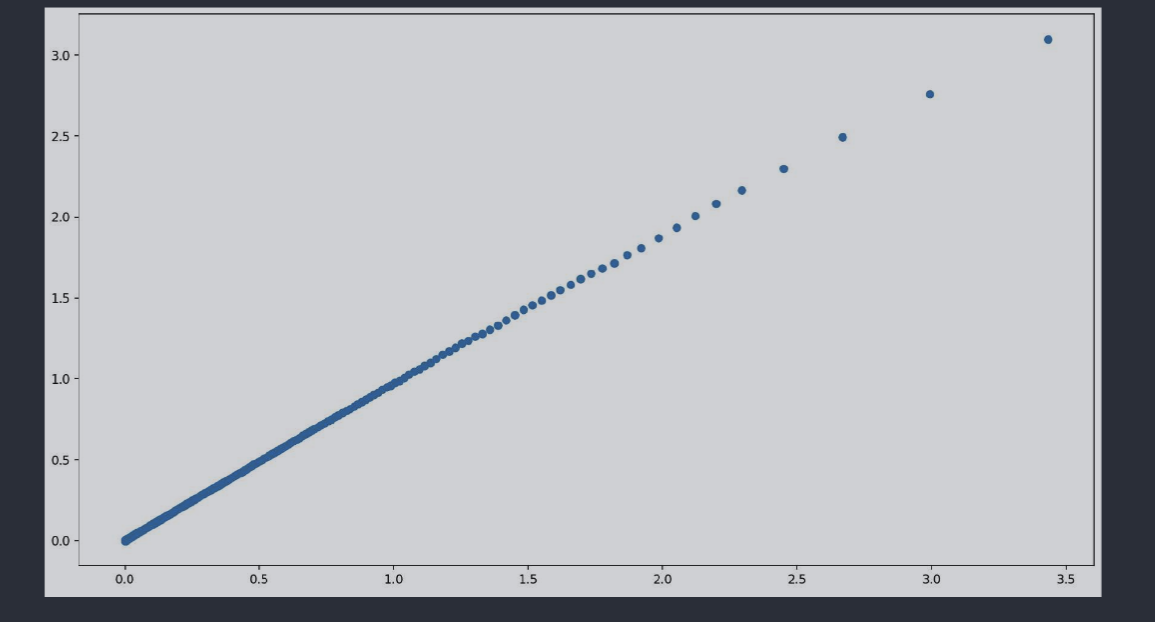 $\text{x axis}: C(v_{1})+C(v_{2})+\dots \text{y axis : }C(v_{1}+v_{2}+v_{3}+\dots)$
cross layer contribution on FFN subvalues
- when subvalue $v$ is added on $x$, $v$ is more helpful to increase token $t$‘s probability if $bs_{t}^v$ is larger.
- for transformers, a layer level or subvalue level vector works both as a query to activate other subvalues and as a value.
this brings us to the next question to answer: in addition to parms directly storing knowledge, any way they can influence other parms?
FFN subvalue activation
-
FFN subvalue activated by layer’s residual output and residual output is a sum of a list of layer-level vectors on prev layers.
$m_{i}^k=ReLU(LN(L_{res_{i}}).FN1_{i}^k+b_{i}^k)$
-
each layer level vectors split into suvalue level vectors.
-
so, each lower layer’s attention/FFN subvalue is a “query” to activate the coeffcient scores of upper layer’s FFN subvalues.
-
for activated FFN subvalues, eqn becomes:
$m_{i}^k=LN(L_{res_{i}}).FN1_{i}^k+b_{i}^k$ with $L_{res_{i}}=L_{in_{0}}+ATTN_{0}+FFN_{0}+\dots+ATTN_{i}$
- each previous layer’s vector is contributing to compute the subvalue’s coefficient score.
- a vector’s contrib can be shared into diff subvectors, letting us compute which vector ACTUALLY contributes. so, we’re trying to figure out who actually gets the credit.
we know, $L_{res}=L_{in}+ATTN$. what we want to be able to answer is:
if the final score for the next token “Delhi” is 4, how much of it came from the input and how much from attention?
here, $L_{res}$ is the contribution score ie the final value we want to explain and then there’s a coefficient score that helps us measure the “strength” of the signal/vector before normalisation.
for eg, $L_{in}$ has coefficient score of 2 and $ATTN$ has coefficient score of 1.
total coefficient score=3
$L_{in}$ gets 2/3 of final score and ATTN gets 1/3.
however, we can’t directly say that because we are using LayerNorm for the $L_{res_i}$, making it non linear.
so, for standard LayerNorm,
group all multiplicative terms and all constant terms and you get:
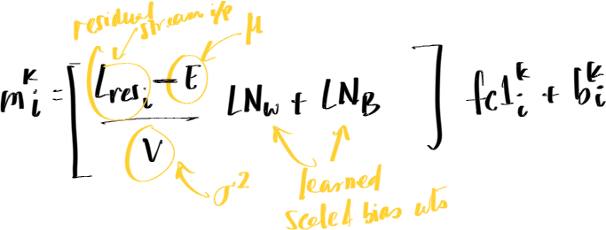
$$m_{i}^k=\frac{{L_{res_{i}}.K_{i}^k}}{V}-\frac{{E\lambda_{k}}}{V}+B_{i}^k$$
where, $K_i^k=LN_{w}fc1_{i}^k$ , $\lambda_{k}$ is sum of all dimension scores of $K_{i}^k$ and $B_{i}^k=LN_{b}.fc1_{i}^k+b_{i}^k$
- for each FFN subvalue, $K_{i}^k$ and $B_{i}^k$ are fixed.
- the only thing changing are $L_{res_{i}}$ and subsequently, $E$ and $V$ .
- In the equation, the bias term is dominated by the numerator of $\frac{{L_{res_{i}}.K_{i}^k}}{V}$.
- if the dot pdt is big: neuron fires strongly
- if the dot pdt is weak, neuron fires weakly
- to find which part of the residual stream switched the neuron on, we just calculate the inner dot product ie $Score=Vector.K_{i}^k$ where vector maybe output of attn head.
- roughly linear relation
Assumptions:
after reading the paper, i got to know there are a few terms/assumptions that are paper specific and do not translate 1:1 to the field of mech interp. clearing that out.
| Term | Standard concept | Nuance |
|---|---|---|
| subvalues | neuron(FFN) or features | |
| knowledge is stored in FFNs | ”key-value” memories | Geva et al first layer acts as pattern/key and second layer writes associated content/value. |
| contrib=prob increase | logit lens/direct logit attribution | standard, but limited. here, we ignored the fact that some heads can suppress probs of incorrect tokens and circuit components which don’t directly affect output but prepare data for future layers. |
| FFNs refine “non linearly” | linear updates | FFN contains non linearity in the form of ReLU or GELU, but with the residual stream, it has a STRICTLY linear addition relation. they “read” a direction and “add” a new vector |
| features are “evident” | superposition/polysemanticity | single parm doesn’t have single meaning. models generally use superposition to store multiple incompatible features in a single neuron |
conclusion
The residual stream is the central highway of transformer computation—a single, persistent space where information accumulates layer by layer. What struck me most is the linear nature of it all: attention heads and FFNs read from this stream, transform information, and write back via simple vector addition. Yet from this linear substrate emerges the non-linear complexity we observe. These notes capture my initial mapping of the territory; a more intuitive, guided exploration—connecting the mathematics to visual intuition—will follow in a proper blog post soon.