Day 0

Terminology

Policy:

Rule used by agent to decide what action to take
- stochastic
  - $a_t \sim \pi(\cdot|s_t)$
  - at any given moment $t$, agent looks at current situation $s_t$ . Instead of a fixed move, it has a choice of moves, each with a specific probability. randomly picks move $a_t$ based on probability.
  - two types:
    1. Categorical
      - discrete action spaces. classifier over discrete actions.
      - Input: observation -> some layers -> logits for each action -> softmax to get probs
      - Sampling: given the prob for each action, sample.
      - log likelihood: denote last layer probs as $P_{\theta}(s)$. vector with many entries=actions. log likelihood for action $a$ into vector $\log \pi_{\theta}(a|s)=\log[P_{\theta(s)}]_{a}$
    2. Diagonal Gaussian Policies
      - multivariant gaussian distrib described by mean vector $\mu$ and covariance matrix $\sum$.
      - diagonal gaussian distrib special case where cov matrix has only diagonal entries. $\therefore$ vector representation
      - 2 ways to represent as vectors:
        
        single vector of $\log(\sigma)$ (SD)
        
        neural net that maps from states to $\log_{\theta}(\sigma)$
- deterministic
  - $a_{t}=\mu(s_{t})$
  - action exactly determined by state, no randomness
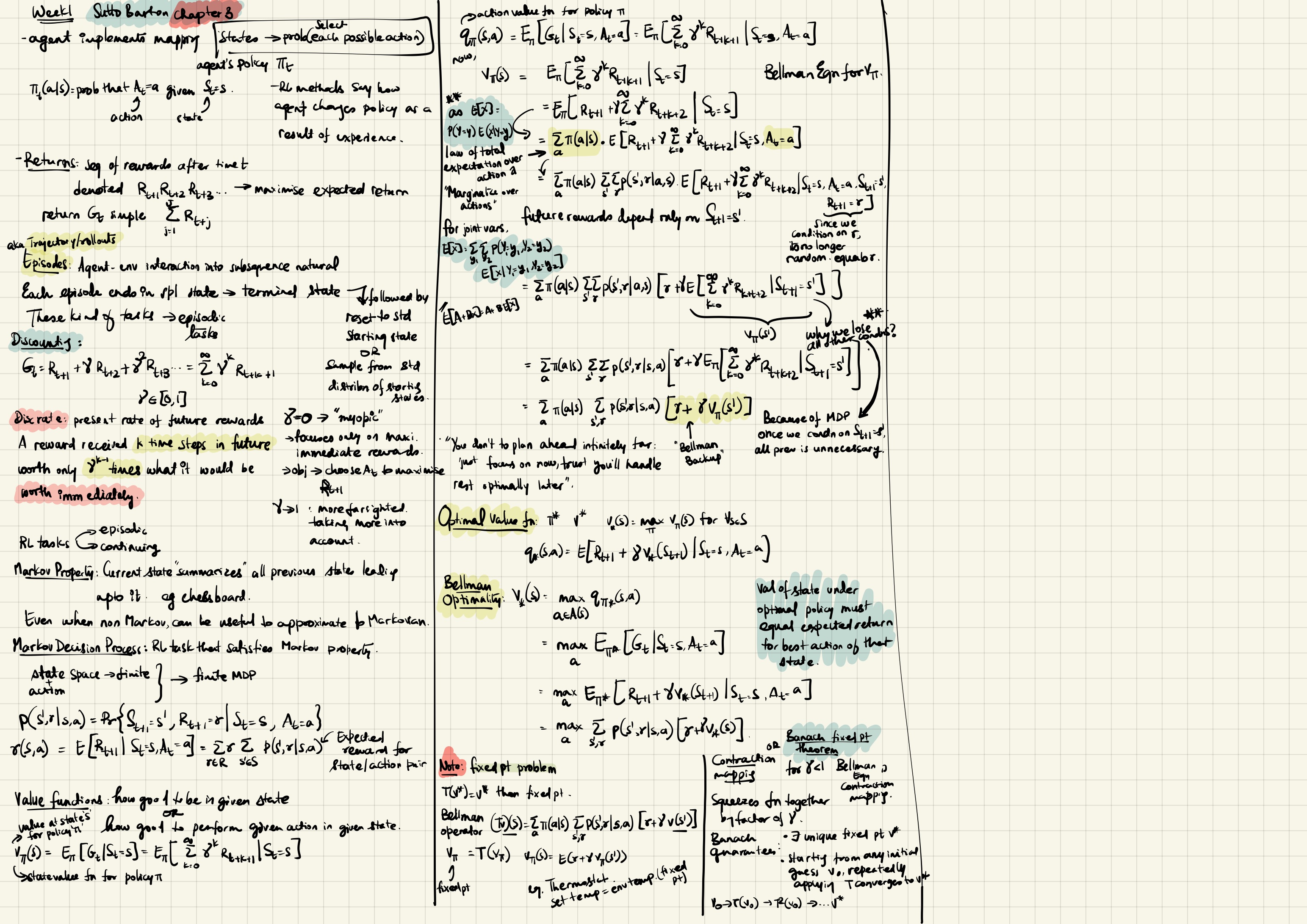
Returns
- finite horizon undiscounted return: sum of rewards obtained in a fixed window of steps $$R(\tau)=\sum_{t=0}^Tr_{t}$$
- infinite horizon discounted return: sum of all rewards ever , discounted by how far off they’re obtained. “reward received k time steps in future worth only $\gamma^{k-1}$ times what it would be worth immediately”. $$R(\tau)=\sum_{t=0}^\infty \gamma^tr_{t}$$
Trajectory
- $\tau$ sequence of states and actions
- $s_0$ sampled randomly from start state distribution, denoted by $\rho_{0}$ is $s_{0}\sim \rho_{0}(\cdot)$

RL Problem

maximisation of expected return over a given horizon.

for stochastic env transitions and policy, probability of T-step trajectory $$P(\tau|\pi)=\phi_{0}(s_{0})\prod_{t=0}^{T-1}\pi(a_{t},s_{t})P(s_{t+1}|s_{t},a_{t})$$

the expected return is $$J(\pi)=\int_{\tau}P(\tau|\pi)R(\tau)=\mathbb{E}_{\tau \sim \pi}[R(\tau)]\quad \text{expected Reward for trajectory }\tau\text{ following policy }\pi$$

the central optimisation problem in RL can be then expressed by as $\pi^*=\mathbb{\text{argmax}}_{\pi}J(\pi)$ where $\pi^*$ is the optimal policy.

Value Functions

value of state/state-action pair ie expected return if you START in that state or state=action pair and act on policy.

types:

on policy value function: expected return for start state s and always follows policy $\pi$ $$V^\pi(s)=\mathbb{E}_{\tau\sim \pi}[R(\tau)|S_{0}=s]$$
on policy value action function: expected return for start state a and arbitrary action a(may not be on policy) and THEN forever act on policy $\pi$ $$Q^\pi(s,a)=\mathbb{E}_{\tau\sim \pi}[R(\tau)|S_{0}=s,A_{0}=a]$$
optimal value function: max value of $V^\pi(s)$ subject to $\pi$ acting always according to optimal policy
optimal value action function: max value of $Q^\pi(s,a)$ subject to pi, first on arbitrary action a and then forever according to optimal policy

Question

When we talk about value functions, if we do not make reference to time-dependence, we only mean expected infinite-horizon discounted return. Value functions for finite-horizon undiscounted return would need to accept time as an argument. Can you think about why? Hint: what happens when time’s up?

Solution

When time’s up, $v_{t}(s)=0$ for all states. since there is no more reward to be gained as time is over. so, $v_1(s)\ne v_{10}(s)$. that’s why.

Bellman Function

RL Mastery-2

Advantage function

how much better than others on average <- useful for policy gradient methods

$$A^\pi(s,a)=Q^\pi(s,a)-V^\pi(s)$$

RL Mastery Notes — Week 1

On This Page